Decision-Based Valuation method
Last Updated November 26, 2018
The Decision-Based Valuation method, proposed by J.B. Stander in 2015, seeks to estimate the relative contribution of data (similar to the Business Model Maturity Index method) while also accounting for data attributes (such as quality and frequency of collection) relative to the decision being made.
The Decision-Based Valuation method is similar to the Business Model Maturity Index method in that it assesses data’s value in terms of the contribution data make to the outcome. The Decision-Based Valuation method also adjusts the value of the data based on how fit-for-purpose the data are by accounting for
- how the value of the data may change over time,
- the quality of the data relative to its end use, and
- the degree of effort needed to convert data into usable information.
This method takes a top-down approach by identifying the use case first and then determining which data are needed to inform the decision (Figure 1).
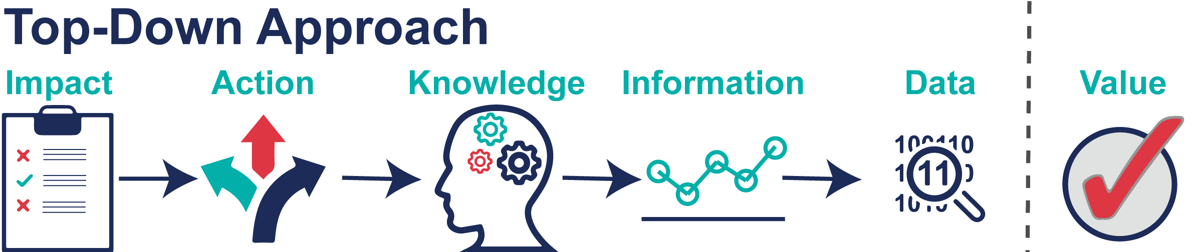
Figure 1: The Decision-based Valuation method takes a top-down approach to estimate the contribution of data to achieving the desired impact.
Decision-based Valuation method
The Decision-Based Valuation method progresses from (1) identifying a desired outcome and its potential impact, (2) developing a series of use cases, with the data required, to achieve the desired outcome, (3) adjusting the value of the data based on how fit it is for this purpose, and (4) estimate the costs, (5) calculate a return on investment, and (6) using expert judgment to estimate the relative contribution, and value, of data to each use case.
(1) Identify a desired outcome and estimate its potential impact
Clearly articulate a desired outcome that can be quantified in terms of time savings, cost savings, water savings, lives saved, etc. The estimate does not have to be precise and can rely on expert judgment.
(2) Develop use cases and estimate cost and impact
Use cases refer to decisions and strategies that can achieve the desired outcome. For each use case, estimate the implementation cost and the potential impact. The value of the decision should be accounted for over the full life-time of the project.
(3) Adjust value based on how fit-for-purpose data are to inform decisions
The value of the use case is adjusted based on the frequency of data collection and their quality relative to what is needed to make a good decision.
Frequency
Frequency compares how often the data must be collected to inform decision-making. The frequency tolerance is the window around which decision-making will be impaired if data are collected less frequently. The adjustment is:
- if Collected Frequency ? Required Frequency then Data Frequency = 1
- if Collected Frequency < Required Frequency then:
- If Data Frequency ? 0, then Data Frequency = 1
- If Data Frequency < 0, then Data Frequency = 0
Accuracy
Data accuracy is compared with the required accuracy for a use case. The adjustment is:
![]()
When the quality is not known, expert opinion can be used. The recommended categories are:
- 0.2: poor, unusable data
- 0.4: substandard data quality
- 0.6: usable and functional data quality
- 0.8: excellent data quality
- 1.0: perfect data
Quality Modifier
The Quality Modifier ranges from 0 to 2 and is the sum of the Frequency and Accuracy score. The estimated value of the data is adjusted by multiplying it with the quality modifier.
(4) Estimate the costs from data acquisition to decision
Stander uses five distinct categories to estimate costs:
- Labor
- Hardware
- Software
- Utilities (such as building costs, energy costs, and so on)
- Contractual (if the work is being contracted outside of the organization).
If the data are currently used for a single decision point, then the full cost is weighted against the benefit of that decision. However, if the data are used for multiple decisions, then the cost can be equally divided between those decisions. Additionally, infrastructure can be depreciated or amortized annually.
(5) Calculate return on investment and performance value of use cases
The Return on Investment (ROI) is calculated as: ![]()
- ROI > 1: benefits exceeded the cost of the project
- ROI = 1: monetary benefits are equal to the costs.
- ROI <1: the benefits are less than the cost of the project
Note that while the economic ROI might be less than one, the reputational, social, or environmental benefits may still justify the cost of the project. Initially the potential ROI is calculated, but as the project occurs, the actual ROI can be estimated by adjusting according to the Performance Value.
![]()
(6) Assign relative contribution and value of data
The value of the data can be estimated based on their relative importance to the use case. The importance ranges from 0 (none) to 1 (critical).
![]()
The value of the data can also be weighted by the level of difficulty to transform the data into usable information, such that data are more valuable with lower processing time.
![]()
The value of the data is multiplied by its relative contribution and divided by its processing value:
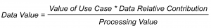
The ROI for data is estimated by dividing the adjusted value by the data’s cost.
Example application
IoW Alfalfa grows alfalfa and is exploring ways to save money while maintaining productivity. Specifically, they are attempting to reduce energy costs by 10 percent.
(1) Identify a desired outcome and estimate its potential impact
IoW Alfalfa wants to reduce energy costs by 10%. Energy costs have increased as groundwater levels have declined. Currently, it costs IoW Alfalfa $0.21 to pump each AF of water one foot in elevation. IoW Alfalfa spends $2.52M annually to pump 60,000 AF from a depth of 200 ft. If they reduce energy costs by 10%, IoW Alfalfa could save $252,000 annually.
(2) Develop use cases and estimate cost and impact
IoW Alfalfa developed several use cases to help them achieve a 10% energy reduction (Figure 2).
- Groundwater Recharge – data can inform how much, when, and for how long fallowed fields should be flooded to maximize groundwater recharge.
- Irrigation Efficiency – data can inform the impact of different irrigation technologies and strategies to reduce the amount of water needed for irrigation.
- Alternative Water Sources – data can inform whether there are cheaper, alternative water sources.
- Alternative Energy Sources – data can inform the energy potential of solar panels, wind turbines, natural gas, or other alternative energy sources to supplement electricity.
- Crop rotation – data can inform the impact of growing alternative, less water intensive crops.
The data required for making these decisions include:
- Crop type: What crops are on the field? What other crops are an option?
- Crop water use: How much water does each crop use? What crops are flood resistant?
- Groundwater levels: What are current groundwater levels? What is the trend? How does it respond to on-farm flooding?
- Energy prices: What is the cost for other energy options (hydropower, solar, wind)?
- Soil moisture: What is the soil moisture? How does that vary by soil type and crop water use?
- Streamflow: What are surface water and groundwater interactions? Is surface water available to supplement?
- Water rights: Are there available surface water rights? Groundwater rights?
- Wastewater utilities: Are there wastewater or reclaimed water options?
- Weather data: When and how much does it rain? What is the evapotranspiration?
Because this method is more intensive than the Business Model Maturity Index method, we will only apply the Decision-Based Valuation method to the groundwater recharge use case.
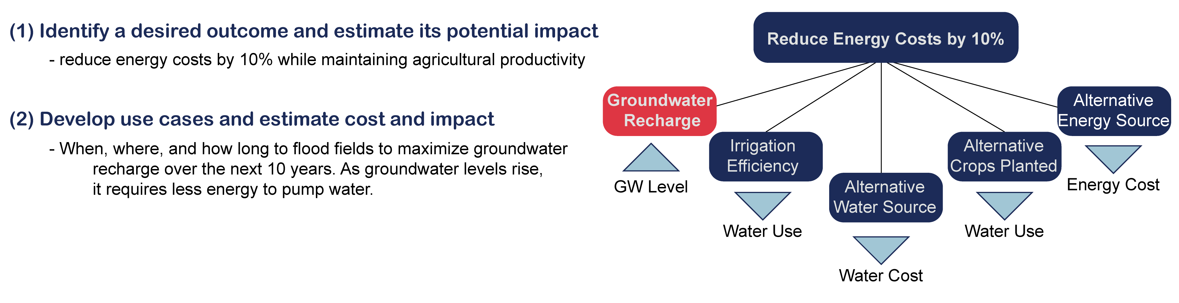
Figure 2: The first steps are to identify a desired outcome and potential use cases. For the purpose of this example, IoW Alfalfa will only explore the groundwater recharge use case.
IoW Alfalfa’s next step is to document the ability of the use case to meet the 10% energy reduction goal. Here, groundwater recharge has the potential to raise water levels by 1 to 10 feet per year for a total of 10 to 100 feet over the 10 year period. This would result in between $12,600 (for 1 foot rise in groundwater levels) and $126,000 (for 10 feet) in energy savings per year (1-5% of the desired energy savings), resulting in between $0.693M and $6.93M savings in pumping costs. By year 10, annual energy used for pumping would be reduced by 10 to 50% (Figure 3).
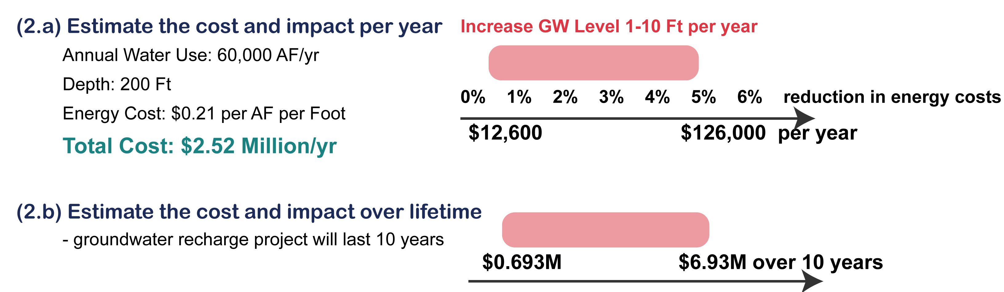
Figure 3: The estimated value of increasing groundwater level per year (top) and across years (bottom). Lower values are realized if groundwater levels only rise 1 foot, higher values for 10 feet, per year.
(3) Adjust value based on how fit-for-purpose data are to inform decisions
Frequency
IoW Alfalfa would like to revisit groundwater recharge decisions every 5 business days. Data more than two days old would impact decisions, meaning their tolerance for decision-making is 2 days, while the actual data collection frequency is daily. Because the Collected Frequency ? Required Frequency, the Data Frequency = 1.
If the data were collected every 14 days the Data Frequency score would be zero because data frequency is below zero:
![]()
Accuracy
IoW Alfalfa knows the accuracy of their groundwater sensors are ± 0.2 ft. However, the decision only requires an accuracy of ± 1 foot. For this decision, the accuracy is 0.8 because Accuracy = (1 Ft – 0.2 Ft)/1 Ft. If the required accuracy were 2 ft, then the data accuracy score would be of 0.9.
Quality Modifier
Since the frequency and accuracy of the groundwater data are fit-for-purpose, the Quality Modifier is 1.8 (Frequency Score + Accuracy Score). Assuming the average annual groundwater level rises 5 ft per year, the average cost savings is $63,000 (2.5% annual savings). Once adjusted, the estimated value of the data increased to $113,400 per year ($63,000 * 1.8) (Figure 4).
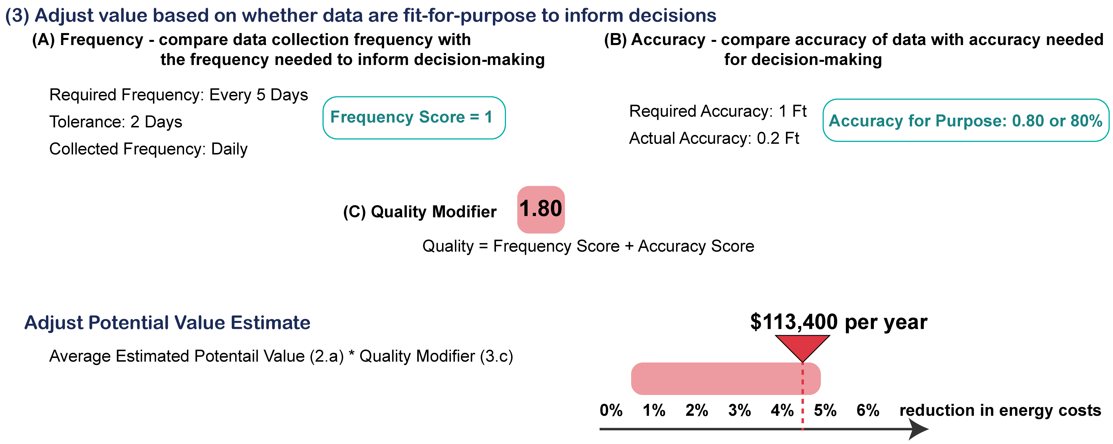
Figure 4: Adjust the value of the data based on collection frequency and accuracy
(4) Estimate the costs from data acquisition to decision
IoW Alfalfa estimated the costs of the groundwater recharge project:
- Labor: $3,000 to set up sensors in the first year and $2,500 to process the data annually.
- Hardware: The majority of the data were public (free). However, 3 new sensors were installed in year one at $10,000 per sensors. The sensors cost an additional $800 to maintain and operate annually. The data server costs $3,000 in year one.
- Software: All analyses was done using free and open software.
- Utilities: The additional energy cost for the server is $500 per year.
- Contractual Fees: None.
The first year is the most expensive at $39,000. Each subsequent year costs an additional $3,800. By the end of year 10, total costs will amount to $77,000 (Figure 5).
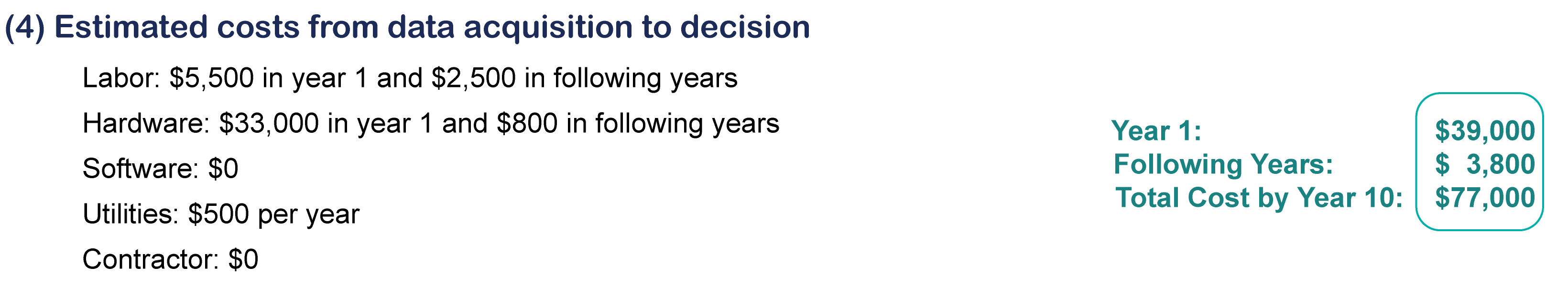
Figure 5: Estimated costs to implement the groundwater recharge project.
(5) Calculate return on investment and performance value of use cases
The ROI for this use case ranges from 2.91 in Year 1 to 15.49 in Year 10 (groundwater levels now 50 feet higher). The overall ROI over the 10 year period is 85.2 ($6.24M/$0.077M) (Figure 6). IoW Alfalfa revisited this estimate after groundwater levels rose by only 3 feet in Year 1 with energy savings of $68,040. The realized ROI decreased to 2.33 in year 1 and 51.12 over the entire 10 year period (groundwater levels now 30 feet higher).
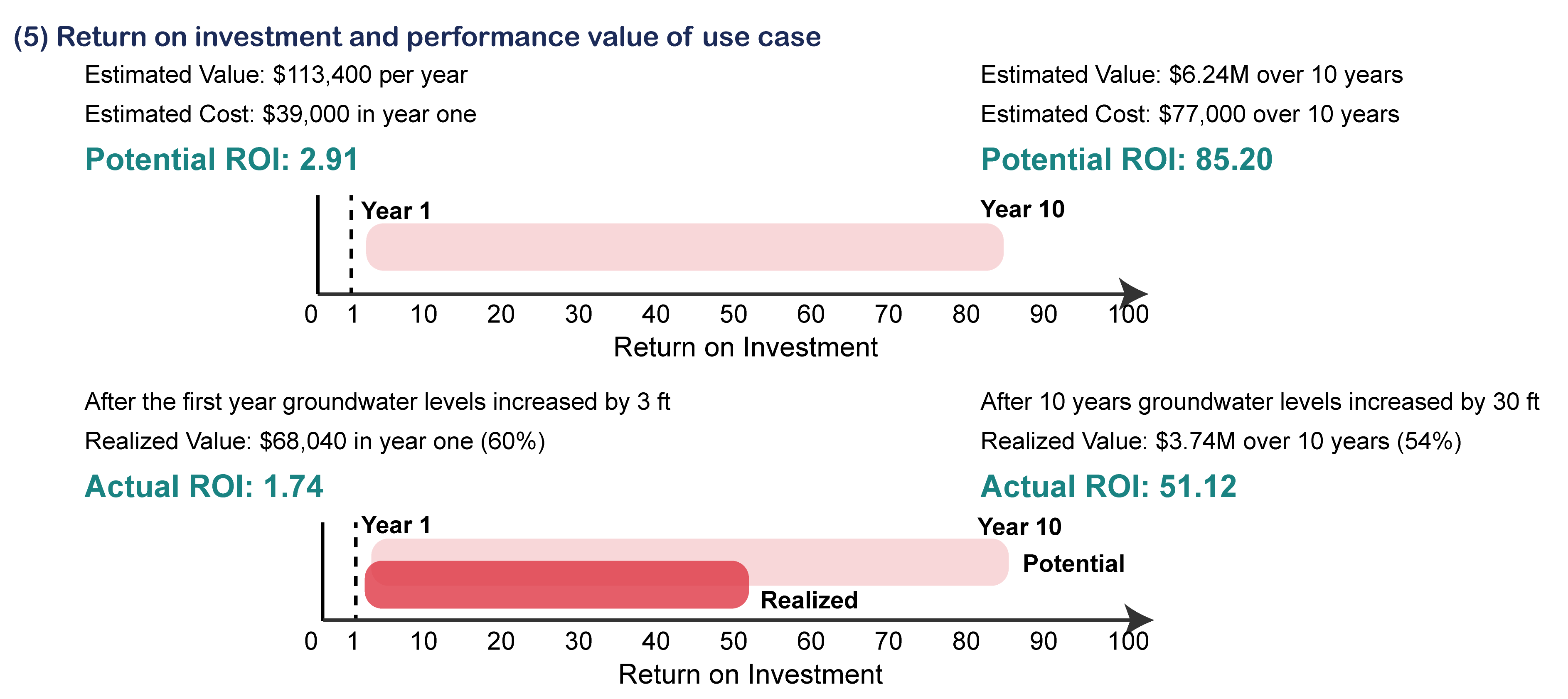
Figure 6: The estimated potential ROI ranged from 3.49 in Year 1 to a 97.2 after 10 years. The realized groundwater levels produced an ROI of 2.33 in year 1 and 52.13 after 10 years.
(6) Assign relative contribution and value of data
The relative importance of each data source were estimated using expert opinion. The sum of the relative importance was 5.25 (Table 1). The relative contribution of groundwater level data, for example, was 0.19 (1.0/5.25). The realized value of groundwater level data in year 1 was $68,040*0.19 = $12,960 (Figure 7). It took IoW Alfalfa 3 hours to collect data from various sources and 10 hours to clean, combine, and convert the data into information (Processing Value = 3.33; 10 hours / 3 hours). This decreased the value of raw groundwater level data to $3,892. The total adjusted value of all data types in year 1 was $20,432, for an ROI of 0.52. However, by year 10 groundwater levels had risen by 30 feet (saving $1.12M in pumping costs) with ROI of 15.35.
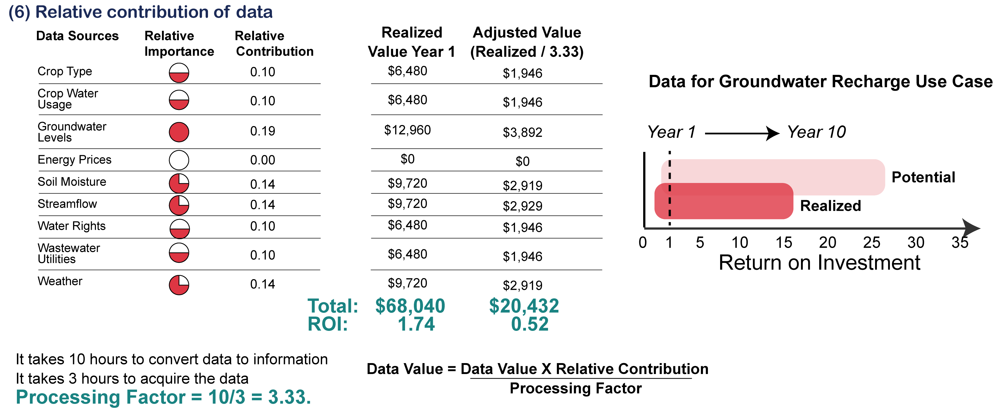
Figure 7: ROI for data used in the groundwater recharge use case.
For more information:
- Cantor, A. et al. 2018. Data for Water Decision Making: Informing the Implementation of California’s Open and Transparent Water Data Act through Research and Engagement.
- Moody and Walsh. 1999. Measuring the Value of Information: An Asset Valuation Approach. European Conference on Information Systems.
- Stander, J.B. 2015. The Modern Asset: Big Data and Information Valuation.