Modified Historical Cost method
Last Updated November 26, 2018
The Historical Cost Method treats data as an asset whose value is at least equivalent to the cost of data collection. This method was modified by Moody and Walsh (1999) to account for the unique attributes of data that cause data to behave differently from traditional physical assets.
The Historical Cost method assumes that data producers behave rationally and will only spend the money needed to acquire an asset if they will receive at least an equivalent economic benefit in the future. The method assumes a return on investment (ROI) is greater than or equal to 1. Data range from potentially having no value to enormous value. For example, some organizations collect data first and decide how to use them later. As a result, sometimes data are never put to use and are only a cost. At the other end of the spectrum, data may be used to inform high impact decisions, resulting in the data being far more valuable than their acquisition cost. Not all data are created equal.
To address these limitations for valuing data, Moody and Walsh (1999) created the Modified Historical Cost method. This method adjusts for the value of the data based on the unique attributes of data, such as the potential for an infinite number of users, the quality of the data, and that duplicate data have zero value. This method has a bottom-up approach where data collected are not tied to an end use, and assumes data are valued in and of themselves, without being tied to impact (Figure 1).
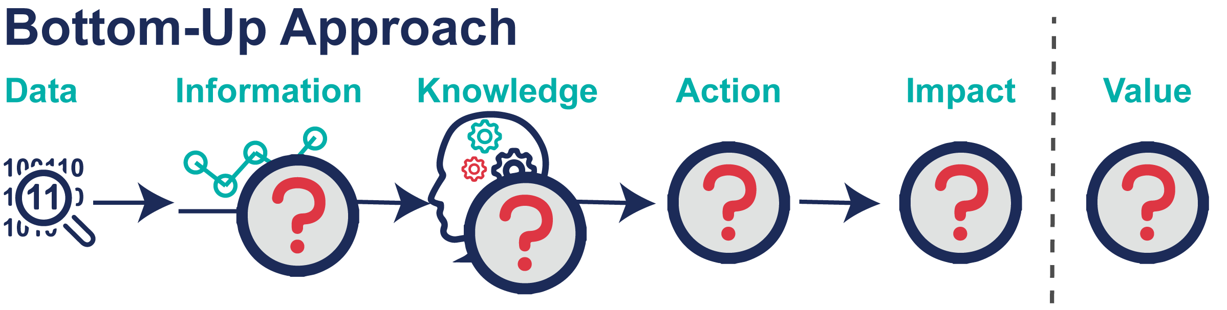
Figure 1: Data’s value is estimated based on data costs and usage attributes.
Modified Historic Cost method
The Modified Historical Cost method adjusts the cost of data collection based on the attributes of the data.
(1) Identify the costs
Data costs include labor, equipment, and infrastructure. There are upfront capital costs to install equipment as well as ongoing operation and maintenance costs. There may be additional data management costs to store, process (such as quality control), and use the data.
(2) Modify value to account for data’s unique attributes
Beginning with the assumption that value is equal to the cost of collection, the following modifications are made to account for data’s unique attributes.
- Redundant data have zero value.
- Unused data have zero value. Data usage can be estimated by number of downloads.
- The more data are used, the greater their value. Therefore, the number of users and data downloads serve as a multiplier to the value.
- The value of the data are depreciated based on data purpose. Operational data for day-to-day decisions have a short life span, while other data may have value for decades based on the decisions they inform. Depreciation rates may be based on the data purpose if usage is unknown.
- Data value should be discounted based on its accuracy (or perceptions of accuracy). Similar to the Decision-Based Valuation method, the ranking may vary between 0 (poor data) to 1 (excellent data).
(3) Return on investment range
Each of the aforementioned adjustments changes the value (and return on investment) of the data. Mapping how the value of data changes with each modification can inform value sensitivity to redundancy, usage, depreciation, and quality.
Example application
IoW Water Utility collects operational data from sensors to inform day-to-day operations. IoW Water Utility also uses public precipitation and water quality data to inform broad decision-making. Twenty five percent of the data collected by IoW Water Utility are for regulatory purposes only.
(1) Identify the costs
The cost to collect data are:
- $10,000 to buy and install a sensor. There are 8 sensors. Total = $80,000
- $1,000 annually to maintain and operate each sensor. Total = $8,000 per year
- $3,000 to buy a data server
- $2,500 to manage and analyze data
- $500 to collect and integrate public data
The total cost in year one is: $86,000. The annual cost for each subsequent year is $4,000. By the end of year 10, $126,000 will have been spent on data with an average of $11,450 spent annually (Figure 2).
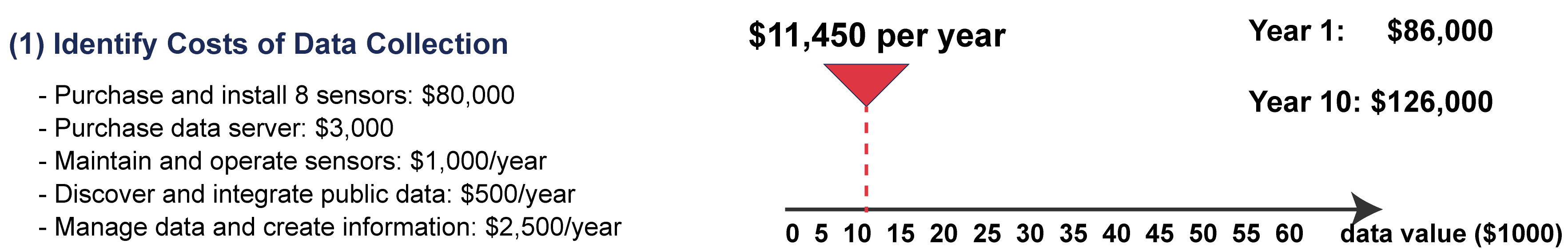
Figure 2: The value of data are equivalent to annual collection costs.
(3) Return on investment range
Once data’s unique attributes were taken into account, the return on investment ranged from 0.63 (value of data to a single user) to 4.77 (value of data to 10 users prior to including depreciation and data quality) (Figure 7). The ROI for the data assuming 10 users and depreciated over time was 3.78. Data usage had the largest impact on the value, followed by depreciation. IoW Water Utility can improve its return on investment by increasing data discoverability and quality, while reducing or eliminating duplicated or unused data.
(2) Modify value to account for data’s unique attributes
- Duplicate Assets. An inventory reveals that 5% of the data are duplicates. Since the value of duplicated data are zero (assumes duplicated data are identical), only 95% of the data can produce benefit, reducing the value to $10,882 annually (Figure 3).
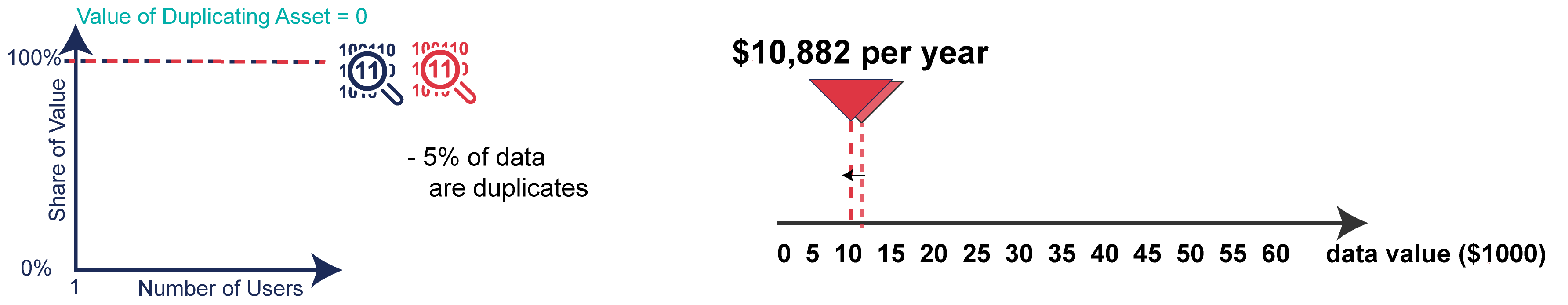
Figure 3: Duplicated data have no additional value.
- Usage. The usage statistics also reveal that there are 10 unique data users with each data user downloading different amounts of data (Table 1). The total value of the data being used is $54,681 (Figure 4).
Data usage statistics reveal that the utility submits but doesn’t use regulatory data. Thus, 25% of the non-duplicated data are not producing value, reducing the data value to $8,161 per year ($10,882*0.75).
Table 1: The value of non-duplicated, non-regulatory data based on usage.
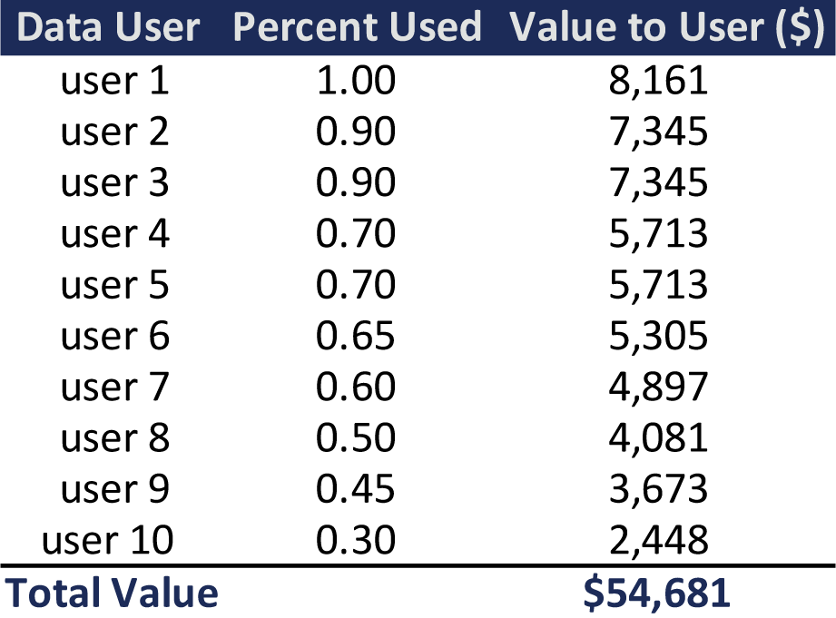
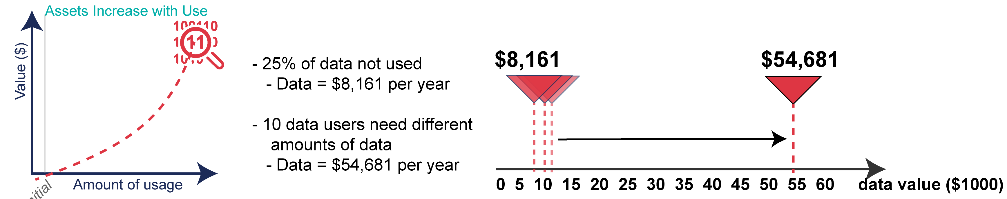
Figure 4: Unused, regulatory data are not valued. The value of data increases in proportion to usage.
- Depreciation. There are numerous methods available for calculating the depreciation value of an asset. IoW Water Utility uses a linear method to depreciate the value of the sensors and the server over their life spans. Sensors last 30 years, resulting in each sensor losing $333 in value annually. By year 10 all 8 sensors combined are only worth $53,330. The data server has a lifespan of 10 years, resulting in the server losing $300 in value annually. By year 10, the server has no value and will need to be replaced the following year (Table 2). The cost of data management does not depreciate over time. With depreciation taken into account, the average annual cost of the sensors and server is $6,197, coupled with an annual labor and hardware costs of $4,000 decreases the average annual cost to $10,196 and reduces the average annual value of to $48,243 (Figure 5).
Table 2: Depreciation of costs over time. All values are dollars.
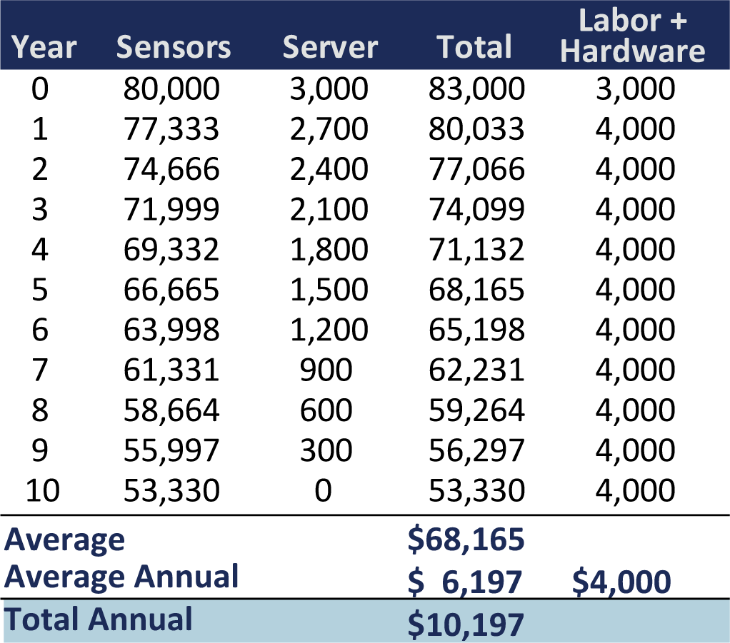
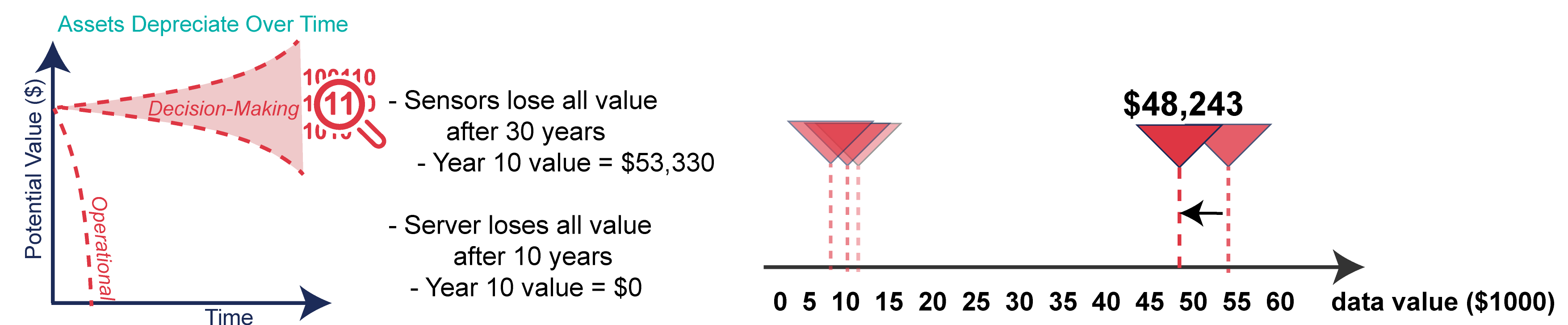
Figure 5: Accounting for depreciation of equipment, the value of the data decreased by 12%.
- Data quality. Data quality can range from 0 (poor) to 1 (excellent). Data quality may be estimated by expert opinion or sensor accuracy. IoW Water Utility’s expert opinion suggests the data are within 20% of actual values, decreasing the depreciated value to $38,594 annually (Figure 6).
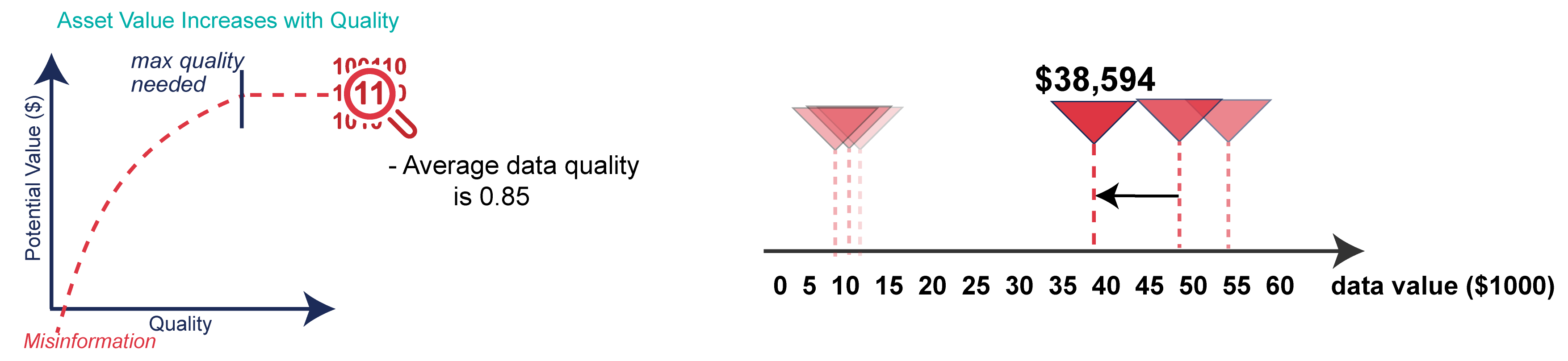
Figure 6: The value of the data reduces to $38,594 after adjusting for quality ($48,243*0.80).
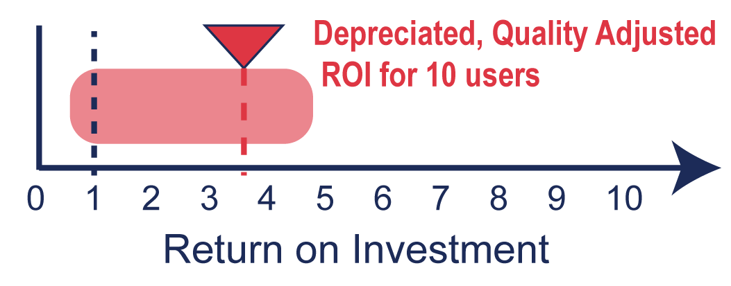
Figure 7: Range of return on investment for IoW Water Utilityccounting for depreciation of equipment, the value of the data decreased by 12%.
For more information:
- Moody and Walsh. 1999. Measuring the Value of Information: An Asset Valuation Approach. European Conference on Information Systems.